Transformer
Transformer
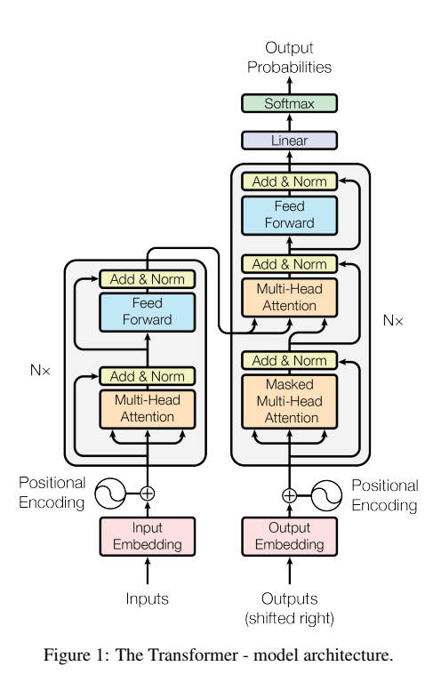
1. Encoder and Decoder
Encoder:
- 6 identical layers (transformer block)
- $output = LayerNorm (x + Sublayer(x))$
- for each layer: multi-head self-attention + position-wise fully connected feed-forward network (MLP)
- residual connection for each sublayer
- layer normalization
- $d_{model} = 512 \ \ \ (d_k = 512)$
Decoder:
- 6 identical layers (transformer block)
- for each layer: masked multi-head self-attention + multi-head self-attention + position-wise fully connected feed-forward network (MLP)
3. Attention
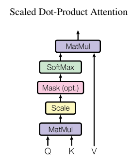
Scaled Dot-Product Attention
query
key-value
The output of attention mechanism is a weighted summary of values. The weight is determined by the similarity between query and corresponding key.
$$
Attention(Q, K, V) = softmax(\frac{QK^T}{\sqrt{d_k}})V
$$
How to measure the similarity between query and key?
The dot-product represents the similarity of two vectors:
$$
cos \alpha = \frac{a \dot \ b}{|a|\dot \ |b|}
$$
$|a|\dot \ |b|$ is a constant, while $cos \alpha$ represents the similarity between two vectors, so $a\dot\ b$ can serve as the measurement of similarity. The similarity of orthogonal vectors is 0.
Why the keys are divided by $\sqrt{d_k}$
If $d_k$ is small (so the size of $a, b$ is small, while the dot-product is small), almost no influence
If $d_k$ is large (the dot-product is large as well), the attention value goes to extreme.
Mask
for mask: $Attention = -1e10$
Multi-Head Attention
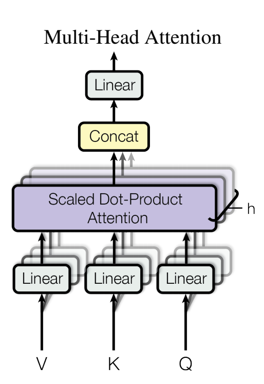 $$
MultiHead(Q, K, V) = Concat(head_1, ..., head_h)W^O
$$
$$
MultiHead(Q, K, V) = Concat(head_1, ..., head_h)W^O
$$
$$
head_i = Attention(QW_i^Q, KW_i^K, VW_i^V)
$$
Multi-head mechanism is similar to multi convolution kernel in CNN
Self-attention
Key, value, query are all the same word embedding.
4. Position-wise Feed-Forward Networks
$$
FFN(x)= max(0, xW_1 + b_1)W_2 + b_2
$$
A simple MLP with one hidden layer. $d_{model} = 512$, $d_{ff} = 2048$
Position-wise operation parallel compute(compare with RNN)
512 - 2048 - 512
5. Embedding
multiply $\sqrt{d_{model}}$ to correspond to the scale of positional encoding
6. Positional Encoding
Positional encoding adds timing information to the model. Otherwise, same words on different position would have the same word embedding.
Can you can a can like a canner can can a can?
If all the words “can” have the same word embedding? …
RNN uses the previous output to generate positional information. It is much slower for parallel computation is not possible.
$$
PE_{(pos, 2i)} = \sin (\frac{pos}{10000^{2i/d_{model}}})
$$
$$
PE_{(pos, 2i+1)} = \cos (\frac{pos}{10000^{2i/d_{model}}})
$$
Moreover, the position embedding of $(pos+k)$ is the linear combination of the position embedding of $(pos)$ and $(k)$. This implies that the position embedding vector contains relative position information. (Which will vanish in the attentio mechanism)
$$
PE(pos+k, 2i) = PE(pos,2i) * PE(k, 2i+1) + PE(pos,2i+1) * PE(k, 2i)
$$
$$
PE(pos+k, 2i+1) = PE(pos,2i+1) * PE(k, 2i+1) - PE(pos,2i) * PE(k, 2i)
$$
7. Residual Link
In all encoder and decoder blocks, Transformer uses residuak link. This helps the network to avoid the problem of gradient vanishing.
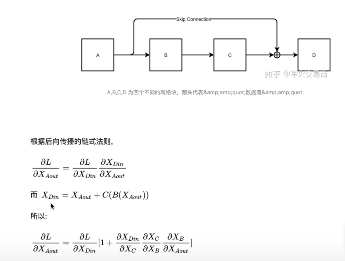
As shown in the figure, “1” in the partial derivative equation ensures the gradient will not come close to 0.
8. Layer Normalization
For data with two dimensions, LN normalize all features of a sample, while BN normalize all samples of a feature.
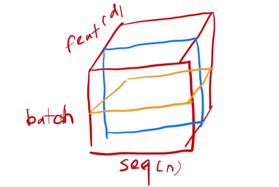
(blue for BN, orange for LN)
For data with three dimensions, LN normalize all the features(embedding) in one sentence(sequence).
Due to the uncertain length of sequences, comparing with hyper-parameter $max_len$, space is padded with 0, and excess part and deleted. The mean value and variance of BN are not stable.(according to LN paper) Therefore, it has a worse performance.
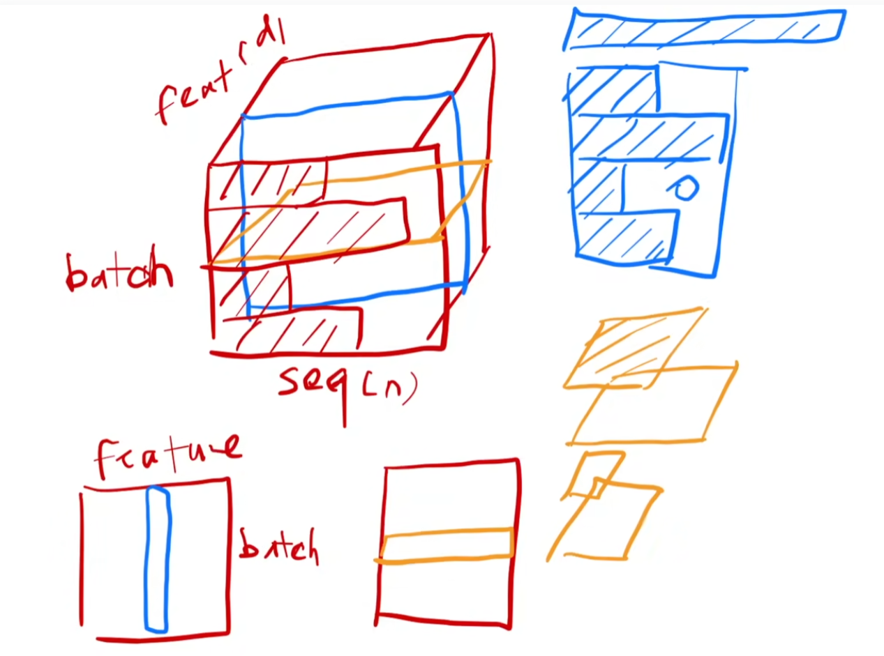
(blue for BN, orange for LN)


