Gaussion Mixture Model
Gaussian Mixture Model GMM 高斯混合模型

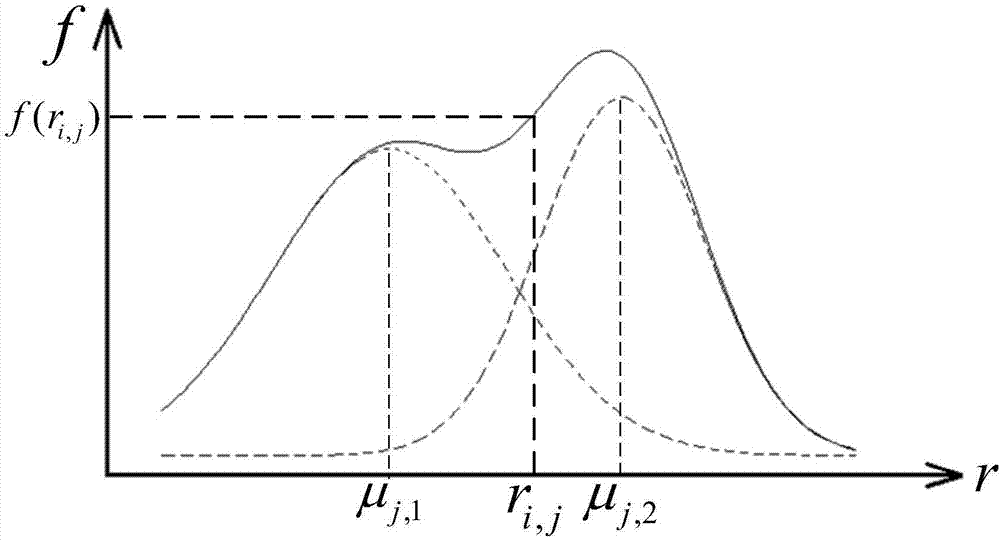
Gaussian mixture model is a combine of multiple Gaussian models. These Gaussian models mixture according to ‘weight’ $\pi$. The picture is a mixture of two models.
GMM
$$
\left{\begin{array}{l}
P(X|c) = \sum\limits_{k=1}^K\pi_kN(x^{(n)}|\mu_k, \Sigma_k) \
N(x^{(n)}|\mu_k, \Sigma_k) = \frac{1}{(2\pi)^{\frac d2}|\Sigma_k|^{\frac12}}exp[-\frac12(x^{(n)}-\mu_k)^T\Sigma^{-1}(x^{(n)}-\mu_k)] \
\sum\limits_{k=1}^K \pi_k= 1
\end{array}\right.
$$
$\pi_k$ – the probability of one example belongs to the $k^{th}$ Gaussian model/the weight of $k^{th}$ model in the mixture model
Attention! GMM is not a convex function and it has local optima(k local optima). What shall we do?
Strategies:
(i) gradient descent
(ii) heuristic algorithm including Simulated Annealing, Evolutionary Algorithms, etc (People hardly use these algorithms nowadays)
(iii)EM algorithm Today’s superstar
EM Algorithm for GMM
Pros and cons
Cons:
- EM algorithm is not a general algorithm dealing with non-convex problem.
Pros:
- No hyper-parameters
- Simple coding work
- Theoretically graceful
EM for GMM
$\gamma_{nk}$ – the probability of $x^{(n)}$ belongs to $k^{th}$ model
$N_k$ – the expectation of #examples belong to $k^{th}$ model
$randomize {\pi_k,\mu_k,\Sigma_k}{k=1\sim K} \
while (!converge) \
{ \
\ \ \ \ \ \ \ \ E-step: \ \
\ \ \ \ \ \ \ \ \ \ \ \ \ \ \ \ \gamma{nk} = \frac{\pi_kN(x_n|\mu_k, \Sigma_k)}{\sum\limits_{k=1}^KN(x_n|\mu_k, \Sigma_k)} \
\ \ \ \ \ \ \ \ M-step: \ \
\ \ \ \ \ \ \ \ \ \ \ \ \ \ \ \ N_k= \sum\limits_{k=1}^K\gamma_{nk} \
\ \ \ \ \ \ \ \ \ \ \ \ \ \ \ \ for(k \ models) \
\ \ \ \ \ \ \ \ \ \ \ \ \ \ \ \ { \
\ \ \ \ \ \ \ \ \ \ \ \ \ \ \ \ \ \ \ \ \ \ \ \ \pi_k^{(new)}=\frac{N_k}{N} \
\ \ \ \ \ \ \ \ \ \ \ \ \ \ \ \ \ \ \ \ \ \ \ \ \mu_k^{(new)} = \frac{1}{N_k}\sum\limits_{n=1}^N\gamma_{nk}x^{(n)} \
\ \ \ \ \ \ \ \ \ \ \ \ \ \ \ \ \ \ \ \ \ \ \ \ \Sigma_k^{(new)} = \frac{1}{N_k}\sum\limits_{n=1}^N\gamma_{nk}[x^{(n)}-\mu_k^{(new)}] [x^{(n)}-\mu_k^{(new)}] ^T \
\ \ \ \ \ \ \ \ \ \ \ \ \ \ \ \ { \
}$
We use soft discrimination in this application of EM algorithm, which means we will compute the probability of each examples belongs to all models. In other applictions, take K-Means clustering algorithm for example, we use winner-takes-all strategy.


